In Using NAM, Part 1, we explored the different types of models and presented the main software and hardware loaders currently available. In this second part, we will present the different NAM model architectures, after a brief introduction to the vocabulary associated with the NAM system. We will then provide a practical overview of the resources required to use NAM models “live.” A downloadable model pack is also included with this article so that you can carry out your own tests with different model architectures, if you wish.
Wavenet, epochs and ESR
NAM is based on a deep learning approach applied to audio: a NAM model will produce an output signal from an input signal after being trained for it. And to do this, NAM relies mainly on the Wavenet system. This was originally developed and perfected by Deepmind (a subsidiary of Google) around 2016, and its first field of application was audio generation and more specifically applications in the field of voice synthesis such as text-to-speech (https://en.wikipedia.org/wiki/WaveNet). From a high-level point of view, Wavenet implemented with NAM makes it possible to predict an output value from an input value through the use of a model. This model is generated by learning from a source data set (“input” file) and a target data set, i.e. the result obtained by sending the source signal to the amp or pedal (which constitutes the “output” file). Learning is achieved through NAM’s “trainer” program, which builds the model through the execution of multiple iterations (a.k.a “epochs“).
The resulting model makes its predictions (i.e., the reproduction of the sound from the captured material) based on a system of layers and using parameters governing the dilations.
In the deep learning system, the process is carried out through successive iterations (epochs) during which the ESR (Error-to-Signal Ratio) is monitored. The closer the ESR is to 0, the more faithful the model is to the original. Achieving a low ESR generally requires a relatively large number of iterations: NAM model creators frequently use up to 800 or 1000 epochs. Beyond a certain number of iterations, a plateau is generally observed at which it is no longer worthwhile to continue training, as the gains become very marginal or zero compared to the time and GPU costs.
Regarding ESR, here are some benchmarks inspired by the MOD Audio page describing best practices for AIDA-X captures (https://mod.audio/modeling-amps-and-pedals-for-the-aida-x-plugin-best-practices/), which I’ve slightly modified to apply to NAM:
- ESR <= 0.01: excellent accuracy, the model is very accurate
- 0.01 < ESR ≤ 0.05: very good accuracy, the model is accurate
- 0.05 < ESR ≤ 0.15: good quality/usability compromise, the model is still fairly accurate
- 0.15 < ESR ≤ 0.35: noticeable differences, can be used but with caution
- ESR > 0.5: very approximate modeling, probably unsatisfactory
- ESR > 0.9: very far off, probably unusable Levels, adjustments and alignments to be checked
We’ll get back to this capture and learning phase in another article in this series.
For your information, NAM models are JSON-formatted files that contain information about the model itself and a metadata section that provides the loader with information about the model:
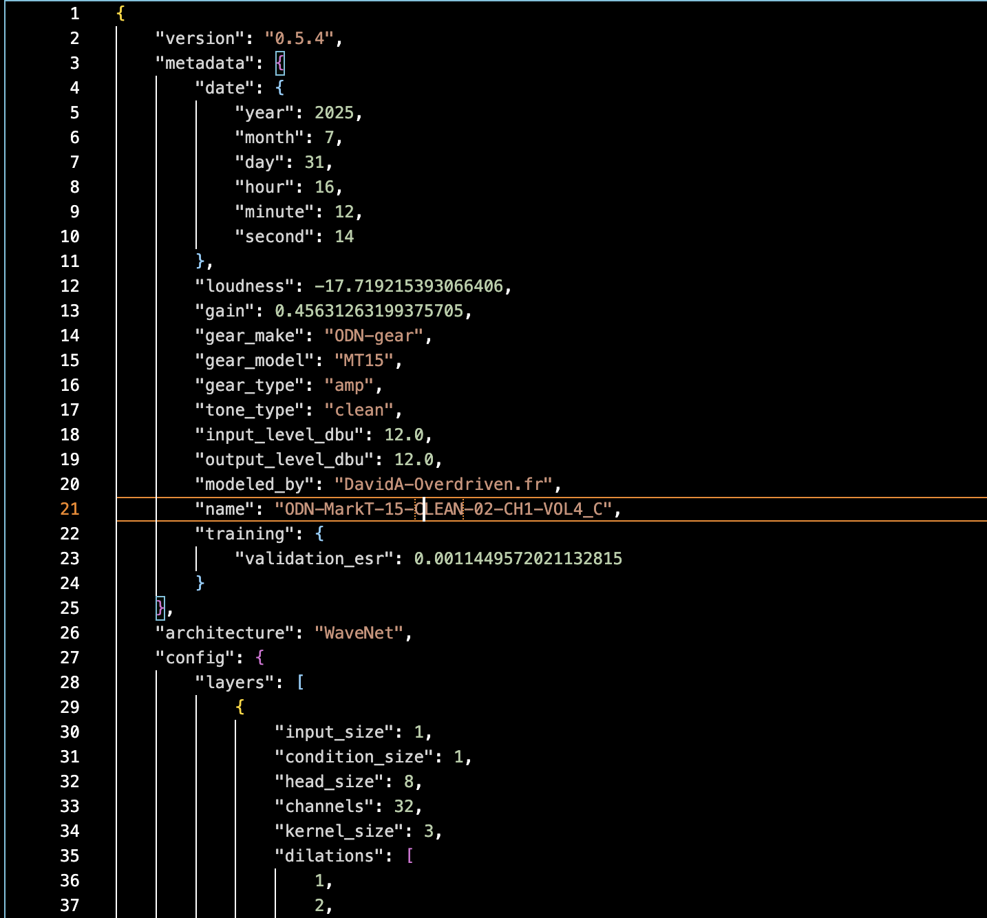
To learn more about the keys used in NAM files, you can explore the contents of .NAM files yourself and consult the small documentation here: https://neural-amp-modeler.readthedocs.io/en/latest/model-file.html#
NAM Architectures
Steve Atkinson has developed 4 sets of parameters, allowing the generation of 4 types of models to address the issue of CPU resources required to use NAM models. In NAM vocabulary, these types of models are referred to as “architectures“. The basic NAM model is considered the “standard” architecture: it offers a very good level of fidelity, but it can be problematic in terms of CPU consumption for users with very low-power or old machines, and especially for proprietary platforms (multi-effects or machines like Raspberry Pi) which frequently rely on processors much less powerful than those of PCs/MACs – or even those of iPhones -, most of the time for reasons of chip costs and associated integration costs. S. Atkinson has therefore introduced lighter variants of architectures: these are the LITE, FEATHER and NANO models. These variants impact the size of the model on disk and in memory, as well as the level of CPU consumption required to run them.
The complexity (and fidelity) of NAM models is defined through the different layers and levels of dilations introduced in the previous section. Ultimately, this complexity can be summarized through the number of parameters managed by the NAM model:
| Architecture | Parameters | Size on disk (approx). |
|---|---|---|
| STANDARD | 13800 | 280-300 KB |
| LITE | 6600 | 141 KB |
| FEATHER | 3000 | 65 KB |
| NANO | 841 | 20 KB |
The NAM user community has also brought out new model architectures, primarily the xStandard and Complex models. The latter seeks to increase the level of fidelity and, unlike the lightweight approach presented in the previous paragraph, it requires significantly more CPU power to run:
| Architecture | Parameters | Size on disk (approx). |
|---|---|---|
| COMPLEX | 90000 | 1.9 - 2.3 MB |
| XSTANDARD | 12400 | 270 KB |
CPU power differences are presented in a later section of this article, and remember, complex models require sufficiently fast machines.
If you’re new to NAM and/or want to explore the rendering and behavior of different model architectures on your own hardware, I invite you to download a starter pack from this link: https://overdriven.fr/overdriven/index.php/nam-models/#MarkT-15_pack_1_8211_extended
This pack contains 7 basic models (1 Clean, 1 Crunch, 3 high-gain, and 2 boosted models with an OD) inspired by an MT 15* amp. This pack can be downloaded from tone3000 (you’ll find the link on the same page), but this version includes—in addition to the Standard, xStandard, and Complex models found on Tone3000—the LITE, FEAHER, and NANO versions, all built from the same re-amped files. As a bonus, this pack includes Genome presets for quick testing. The presets point to the _S (standard) models by default, but you can switch them as you wish.
*See legal notice at the bottom of the article.
Below is a table of the ESRs obtained for the different models in this pack:
| Model name | ESR | Loudness | Tone type |
|---|---|---|---|
| ODN-MarkT-15-CLEAN-02-CH1-VOL4_C.nam | 0.00114 | -17.7 | clean |
| ODN-MarkT-15-CLEAN-02-CH1-VOL4_F.nam | 0.01298 | -17.8 | clean |
| ODN-MarkT-15-CLEAN-02-CH1-VOL4_L.nam | 0.01058 | -17.8 | clean |
| ODN-MarkT-15-CLEAN-02-CH1-VOL4_N.nam | 0.01847 | -17.6 | clean |
| ODN-MarkT-15-CLEAN-02-CH1-VOL4_S.nam | 0.00416 | -17.8 | clean |
| ODN-MarkT-15-CLEAN-02-CH1-VOL4_XS.nam | 0.00477 | -17.6 | clean |
| ODN-MarkT-15-CRUNCH-01-CH2_C.nam | 0.00149 | -17.7 | crunch |
| ODN-MarkT-15-CRUNCH-01-CH2_F.nam | 0.00998 | -18.0 | crunch |
| ODN-MarkT-15-CRUNCH-01-CH2_L.nam | 0.00705 | -17.8 | crunch |
| ODN-MarkT-15-CRUNCH-01-CH2_N.nam | 0.02170 | -18.0 | crunch |
| ODN-MarkT-15-CRUNCH-01-CH2_S.nam | 0.00455 | -17.8 | crunch |
| ODN-MarkT-15-CRUNCH-01-CH2_XS.nam | 0.00434 | -17.9 | crunch |
| ODN-MarkT-15-HIGHGAIN-01-CH2-G3_C.nam | 0.00197 | -18.2 | hi_gain |
| ODN-MarkT-15-HIGHGAIN-01-CH2-G3_F.nam | 0.01500 | -18.5 | hi_gain |
| ODN-MarkT-15-HIGHGAIN-01-CH2-G3_L.nam | 0.00969 | -18.4 | hi_gain |
| ODN-MarkT-15-HIGHGAIN-01-CH2-G3_N.nam | 0.03836 | -18.6 | hi_gain |
| ODN-MarkT-15-HIGHGAIN-01-CH2-G3_S.nam | 0.00656 | -18.4 | hi_gain |
| ODN-MarkT-15-HIGHGAIN-01-CH2-G3_XS.nam | 0.00535 | -18.4 | hi_gain |
| ODN-MarkT-15-HIGHGAIN-02-CH2-G4_C.nam | 0.00235 | -18.3 | hi_gain |
| ODN-MarkT-15-HIGHGAIN-02-CH2-G4_F.nam | 0.01980 | -18.7 | hi_gain |
| ODN-MarkT-15-HIGHGAIN-02-CH2-G4_L.nam | 0.01292 | -18.6 | hi_gain |
| ODN-MarkT-15-HIGHGAIN-02-CH2-G4_N.nam | 0.04332 | -18.9 | hi_gain |
| ODN-MarkT-15-HIGHGAIN-02-CH2-G4_S.nam | 0.00822 | -18.6 | hi_gain |
| ODN-MarkT-15-HIGHGAIN-02-CH2-G4_XS.nam | 0.00732 | -18.3 | hi_gain |
| ODN-MarkT-15-HIGHGAIN-03-CH2-G5_C.nam | 0.00430 | -18.5 | hi_gain |
| ODN-MarkT-15-HIGHGAIN-03-CH2-G5_F.nam | 0.02364 | -18.7 | hi_gain |
| ODN-MarkT-15-HIGHGAIN-03-CH2-G5_L.nam | 0.01586 | -18.6 | hi_gain |
| ODN-MarkT-15-HIGHGAIN-03-CH2-G5_N.nam | 0.05254 | -19.0 | hi_gain |
| ODN-MarkT-15-HIGHGAIN-03-CH2-G5_S.nam | 0.00985 | -18.6 | hi_gain |
| ODN-MarkT-15-HIGHGAIN-03-CH2-G5_XS.nam | 0.00925 | -18.6 | hi_gain |
| ODN-MarkT-15-OD-01-CH1-VOL4_C.nam | 0.00078 | -17.6 | overdrive |
| ODN-MarkT-15-OD-01-CH1-VOL4_F.nam | 0.00521 | -17.6 | overdrive |
| ODN-MarkT-15-OD-01-CH1-VOL4_L.nam | 0.00400 | -17.7 | overdrive |
| ODN-MarkT-15-OD-01-CH1-VOL4_N.nam | 0.01296 | -17.3 | overdrive |
| ODN-MarkT-15-OD-01-CH1-VOL4_S.nam | 0.00209 | -17.6 | overdrive |
| ODN-MarkT-15-OD-01-CH1-VOL4_XS.nam | 0.00263 | -17.7 | overdrive |
| ODN-MarkT-15-OD-02-CH1-VOL4_C.nam | 0.00087 | -17.5 | overdrive |
| ODN-MarkT-15-OD-02-CH1-VOL4_F.nam | 0.00720 | -17.4 | overdrive |
| ODN-MarkT-15-OD-02-CH1-VOL4_L.nam | 0.00381 | -17.6 | overdrive |
| ODN-MarkT-15-OD-02-CH1-VOL4_N.nam | 0.01860 | -17.2 | overdrive |
| ODN-MarkT-15-OD-02-CH1-VOL4_S.nam | 0.00262 | -17.6 | overdrive |
| ODN-MarkT-15-OD-02-CH1-VOL4_XS.nam | 0.00328 | -17.6 | overdrive |
The suffixes used in the table correspond to:
- _S: Standard
- _XS: XStandard
- _C: Complex
- _L: Lite
- _F: Feather
- _N: Nano
Two observations can be made when reading this table:
- The most complex architectures allow for the lowest ESRs (the most accurate models).
- High-gain models (and worse, fuzz models, which are not shown in this example) have higher ESRs than clean or crunch models: these types of sounds are indeed more complex to model.
If you test the sample pack, you should notice some fairly obvious differences, for example, starting with the standard and moving down to Lite, Feather, and then Nano. However, the Lite and Feather models can remain quite good in terms of rendering and can already produce good results.
Last point: in the case where we would like to use several NAM models simultaneously (scenario of one model for an overdrive and another model for an amp), we could consider using light or feather models for the pedal part, the sounds being less complex to model than those of an amp…: the lite or feather models could therefore be enough to produce good results…
A few metrics…
To appreciate the differences between the NAM architectures discussed above, this section presents the results of null tests and the results obtained by carrying out frequency response measurements between the different architectures used for the same model. Caution, null tests are particularly sensitive and can easily break, they are presented here in the context of a very limited comparison (between architectures of the same NAM model) and in a very specific framework:
- Comparison of the amp’s DI to different versions of the same NAM model in complex, standard, etc.
- Model re-captured under the same conditions as the reference DI recording (MT15 Lead Gain 3)
- All recordings are made at the native frequency of 48 kHz
- Standard NAM plugin in raw mode, calibration performed manually (same DI level sent to the amp and the model)
- Manual alignment of tracks to the sample in LogicProx, dual LUFS-I measurement by Logic Multimeter and Fabfilter L2
- The “AMP to AMP” compares two recordings on the reference track’s amp, with inverted phase, and provides a benchmark
- The guitar track used includes chords and note-by-note playing, lasting approximately 40-50 seconds: better LUFS values can be obtained by restricting the comparison to shorter sections, with fewer transients (for example: chord fading for a few seconds), but the comparison then becomes—in my opinion—very partial.
- results are normalized to peak mode at –12 dBFS.
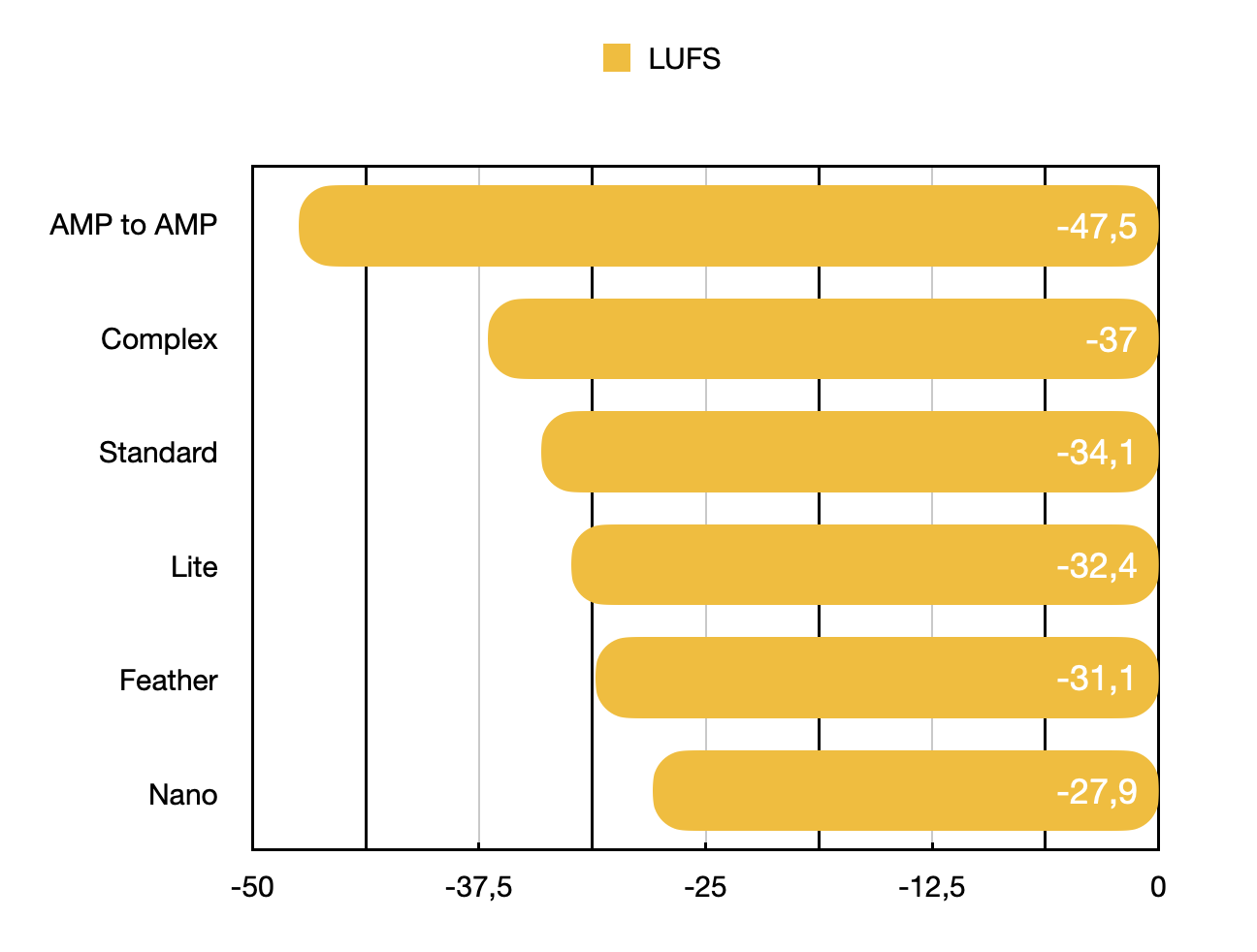
The LUFS-I values and ESRs of the test models are as follows:
| Amp & Model to Amp | LUFS | ESR |
|---|---|---|
| AMP to AMP | -47,5 | - |
| Complex | -37 | 0,0054 |
| Standard | -34,1 | 0,0166 |
| Lite | -32,4 | 0,0230 |
| Feather | -31,1 | 0,0325 |
| Nano | -27,9 | 0,0505 |
Note: this is an example of values achieved in a given context for a particular NAM model: we can compare the LUFS-I values of the test with each other, but it is useless to use the absolute values to compare them with other null tests that you can find on the net. These values can vary by using another model (another amplifier for example), with models calculated in different conditions or with a different test set….
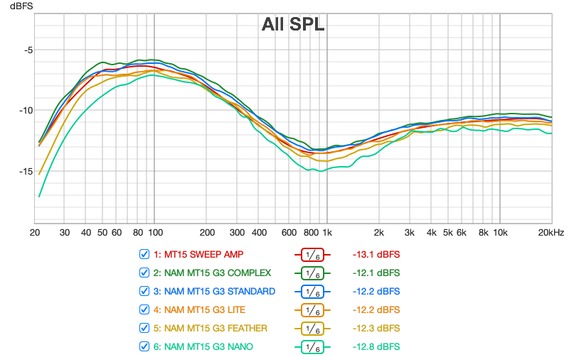
The second set of measurements is carried out using the REW software: these are frequency response measurements of the amplifier and the different variations of the NAM models, in order to visualize the impact of architectures (and therefore potentially the associated ESR values) on the frequency response of the models. These are 10-second sweeps, in red the sweep of the actual amplifier used. NAM plugin in Raw mode used for all NAM models.
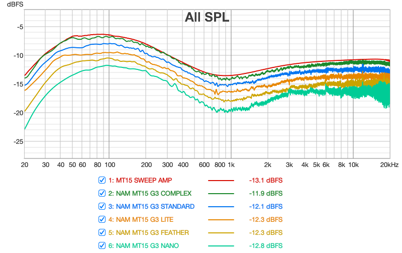
From this first figure, the following observations can be made:
- All the architectures globally reproduce the amplifier’s frequency response curve very accurately.
- All the curves show frequency responses that spread out more and more strongly between 1 kHz and 20 kHz (high-frequency distortion and noise). This phenomenon is relatively contained in the complex and standard models and increases as the architecture complexity decreases.
- The graph confirms listening tests I conducted between the complex and standard models: the complex model has a more precise bass response and is the one whose curve most closely matches the original frequency response.
The following graph shows the same curves by applying smoothing filters to eliminate noise and variations on the high frequency part:
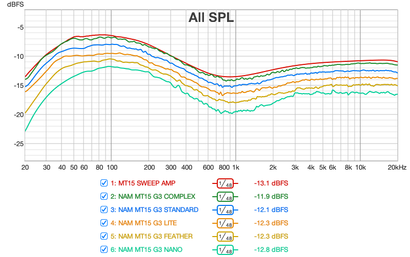
And finally, the same information with less smoothing and separate curves:
CPU resources
The information presented in this section is neither exhaustive nor guaranteed, but rather is intended to provide observations and benchmarks regarding the use of different model architectures—in a specific configuration—on different machine categories, particularly from the perspective of the ability to use models “live,” i.e., to be able to practice, rehearse, and potentially track recordings in real time, either through standalone NAM applications or via a plugin in a DAW. It is strongly recommended that you test the viability of a configuration yourself before purchasing hardware, for your specific context and needs.
The table below presents CPU consumption observations for the standalone Genome application specifically configured with a simple chain using a single NAM model (see the test configuration below); these observations are made manually by reading the information presented by Task Manager on Windows and the Activity Monitor on OSX for tests on Apple hardware. The measurements are observations of “stabilized” values, observed over a few tens of seconds after loading and using a given NAM model, but note that the CPU consumption may fluctuate around the values presented.
The consumption percentages presented are also different between OSX and Windows: on OSX, the maximum CPU consumption is the number of cores * 100: for example, on an 8-core machine the maximum is 800%, and -for example- 110% represents the use of a little more than one core but only represents 110/800 = 13.75% of the total of the machine. Conversely, the values given for Windows are in percentage of the total CPU capacity of the machine: thus 20% on a 4-core machine is indeed 20% of the total CPU capacity, and note that it is also close to the maximum consumption of a single core (100/4 = 25).
Also be aware of the following aspect: less powerful machines can more easily and quickly be disrupted as soon as your system performs other tasks, for example running update systems, antivirus/antimalware scans, indexing processes, etc., which can have the effect of disrupting audio applications such as NAM or Genome standalone (interruptions, crackles, anomalies, etc.). Similarly, if the machine is at the limit of its capacity in the test (i.e. when we are getting close to using a full core of the machine), adding other effects can quickly become problematic: in short, it will be better to have some margin…
Also note the following points, which are important for understanding the presented measurements:
- Genome version used on Mac and Windows: 1.10
- A single NAM model and an IR loader block loaded with a mix of two IRs (100 ms)
- Mono configuration (stereo mode consumes slightly more power)
- Sound card configuration at 48 kHz / 128 samples: in the tests I was able to perform, using higher frequencies results in significantly higher CPU consumption (downsampling/upsampling?)
- Animations disabled in Genome
- Use of two sound cards with ASIO drivers under Windows: SSL2+ MKII and Scarlett 2i2, Core Audio under OSX.
- Genome oversampling disabled (OFF)
- And for reference, the table shows the CPU’s CPU Mark Single Thread score, as reported by https://www.cpubenchmark.net
- 4C, 6C, 8C… : number of cores
| OS/CPU | CPU | Complex | xStandard | Standard | Lite | Feather | Nano |
|---|---|---|---|---|---|---|---|
| OSX/M4 MAX 16C | 4562 | OK (33%) | OK (21%) | OK (20%) | OK (19%) | OK (17%) | OK (17%) |
| OSX/M1 PRO 8C | 3761 | OK (46%) | OK (30%) | OK (29%) | OK (27%) | OK (25%) | OK (23%) |
| Win11/Ryzen 6C | 2871 | OK (11-14%) | OK (3-7%) | OK (4-5%) | OK (3-4%) | OK (2-3%) | OK (2%) |
| Win11/I5-9600K 6C | 2727 | OK (15%) | OK (5%) | OK (5%) | OK (4-5%) | OK (4-5%) | OK (3-4%) |
| OSX/i5-8259U | 2190 | KO** | OK (53%) | OK (49%) | OK (44%) | OK (41%) | OK (37%) |
| Win11/N95 4C | 1927 | KO* | OK (15%) | OK (13%) | OK (12%) | OK (10%) | OK (9%) |
“*”: at the limit, unstable, very sensitive to fluctuations: unusable
“**”: 100% for the host, 85% reported by Genome, at the limit and unstable
Additional CPU information:
- Ryzen 6C: Ryzen 5 5625U 6C
- i5-9600K: i5-9600K @ 3.70 GHz 6C
- i5-8259U: i5-8259U @ 2.30 GHz 4C
- N95: Alder Lake N95 @ 1.70 GHz 4C
Caution/disclaimer: When working with different sampling frequencies (88K, 176K, etc.), with larger buffer sizes, and when working within a DAW (recording, mixing), the required power requirements can vary significantly from those shown in the table. For example, at 176K/512 samples for the oldest Mac on the list (8259U), using the standard model becomes problematic, as does the xStandard on the N95 machine.
On recent and powerful machines, there are no problems running the most complex models (33% for the complex model on the M4 Max, which corresponds to a 2% load for the machine, etc.), and we can see that we can run the standard models on a wide range of machines, at least under the conditions presented in the test.
So, no xStandard or Complex models if we don’t have a powerful enough machine ? Well, there is always the possibility – in the context of recording and creating music tracks – to use your NAM plugin offline in your DAW and to bounce / freeze your tracks, a classic practice when handling somewhat complex projects (in number of tracks and/or number of plugins) or when using plugins that require a lot of resources. The workflow is a little less fluid but it is entirely possible and this puts the use of the most faithful models within your reach even if you do not own a powerful monster….
Conclusion
After an introduction to the fundamental concepts of NAM models and their creation, we presented the different available architectures and their performance in terms of fidelity (ESR). The second part presented the results of observations to provide benchmarks on the hardware and power requirements required to run the different types of models in a live and minimalistic environment. The next article will focus on a key aspect of leveraging NAM models: gain management. Continue reading : Using NAM, part 3
Legal notice
Any and all third party companies and products listed or otherwise mentioned on this site may be trademarks of their respective owners and they are in no way affiliated or associated with Overdriven.fr or the owner of Overdriven.fr. Product names are referenced solely for the purpose of identifying the hardware used in the recording chain for impulse response capture or for guitar or amplifier and pedals sound demonstrations. Use of these names does not imply any cooperation or endorsement. Any use of amplifier, cab or pedal brand name is strictly for comparison and descriptive purpose.
Change log
- Created : 08/12/2025
- Updated : 08/25/2025, added null test and frequency response, link to part 3
Leave a Reply